Binary Search Trees

A binary search tree, sometimes called an ordered or sorted binary tree is a binary tree in which nodes are ordered in the following way:

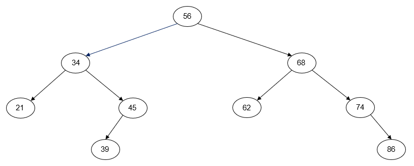
each node contains a key (and optionally also an associated value)
the key in each node must be greater than or equal to any key stored in its left subtree, and less than or equal to any key stored in its right subtree. Depending on the application, duplicate keys may or may not be allowed.

Figure 1: A Binary Search Tree

Performing a left-to-right inorder traversal of a binary search tree will "visit" the nodes in ascending key order, while performing a right-to-left inorder traversal will "visit" the nodes in descending key order.

Binary search trees are a common choice for implementing several abstract data types, including Ordered Set, Ordered Multi-Set, Ordered Map, and Ordered Multi-Map. These ADTs have three main operations:

Insertion of elements
Deletion of elements
Find / lookup an element

Binary Search Tree Insertion

Insertion into a binary search tree can be coded either iteratively or recursively. If the tree is empty, the new element is inserted as the root node of the tree. Otherwise, the key of the new element is compared to the key of the root node to determine whether it must be inserted in the root's left subtree or its right subtree. This process is repeated until a null link is found or we find a key equal to the key we are trying to insert (if duplicate keys are disallowed). The new tree node is always inserted as a leaf node.

Pseudocode for an iterative version of this algorithm is shown below.

Iterative Insertion into a Binary Search Tree Pseudocode

procedure insert(key : a key to insert, value : a value to insert)
    // root     : pointer to the root node of the tree (nullptr if tree is empty)
    // t_size   : tree size  
    // p        : pointer to a tree node
    // parent   : pointer to the parent node of p (nullptr if p points to the root node)
    // new_node : pointer used to create a new tree node
    
    // Start at the root of the tree.
    p ← root
    parent ← nullptr
    
    // Search the tree for a null link or a duplicate key (if duplicates are disallowed).
    while p != nullptr and key != p->key
        parent ← p
        if key < p->key
            p ← p->left
        else
            p ← p->right
        end if
    end while

    // If duplicates are disallowed, signal that insertion has failed.
    if p != nullptr
        return false
    end if
    
    // Otherwise, create a tree node and insert it as a new leaf node.
    Create a new tree node new_node to contain key and value
    
    if parent == nullptr
        root ← new_node
    else
        if new_node->key < parent->key
            parent->left ← new_node
        else
            parent->right ← new_node
        end if
    end if
    
    t_size ← t_size + 1

    // If duplicates are disallowed, signal that insertion has succeeded. 
    return true

end procedure

Binary Search Tree Insertion Example

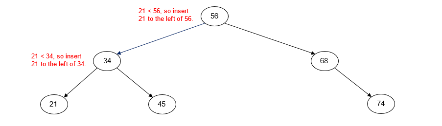
Insert 56 into empty tree
Insert 34
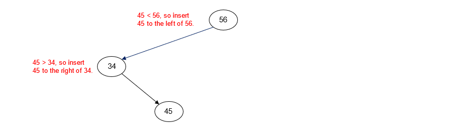
Insert 45
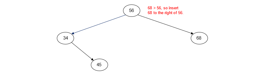
Insert 68
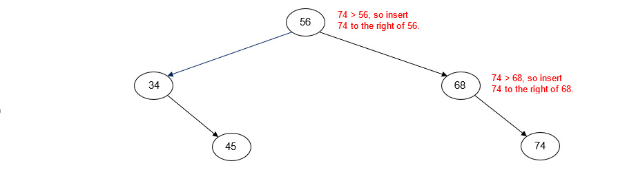
Insert 74
Insert 21
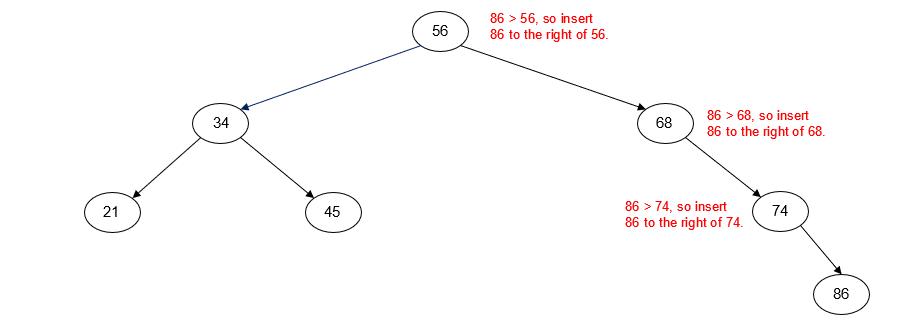
Insert 86
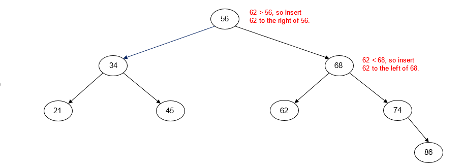
Insert 62
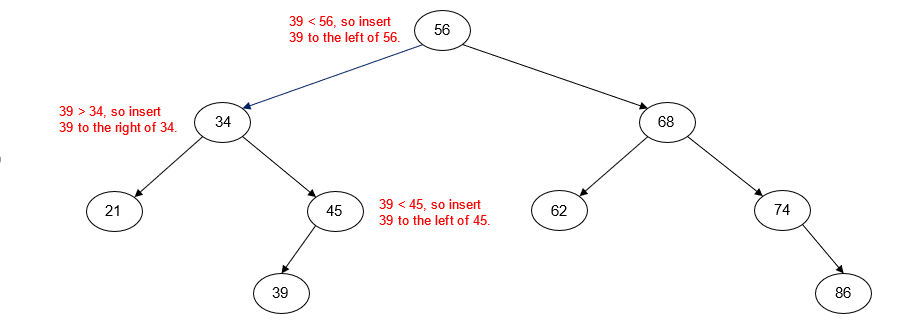
Insert 39

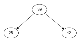
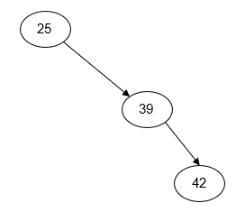
As the example above illustrates, the arrangement of the nodes in a binary search tree depends entirely on the order in which the keys are inserted. For example, if we insert the keys 25, 39, and 42, we could end with any one of five different node arrangements depending on the order in which the keys are inserted:

Figure 2: Alternate Binary Search Tree Arrangments

Insert: 39, 25, 42	Insert: 39, 42, 25	Insert: 25, 39, 42

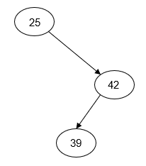
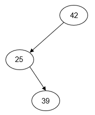
Insert: 25, 42, 39	Insert: 42, 25, 39	Insert: 42, 39, 25

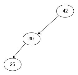All of the trees shown above will produce the same output when traversed using the inorder traversal algorithm.

As the third diagram in each of the rows of Figure 2 shows, if keys are inserted into a binary search tree in sorted order, they will always end up being inserted in the same subtree. The result is referred to as a degenerate binary search tree and is effectively a linked list. This has a negative impact on the complexity of the binary search tree operations (see Complexity below). One way to prevent this problem is with a self-balancing binary search tree such as an AVL tree or a red-black tree. Both data structures are outside the scope of this course.

Binary Search Tree Deletion

Deletion of a node with a specified key from a binary search tree can also be coded either iteratively or recursively. Pseudocode for an iterative version of the algorithm is shown below.

Iterative Deletion from a Binary Search Tree Pseudocode

procedure remove(key : key to remove from the tree)
    // root           : pointer to the root of the binary search tree
    // t_size         : tree size  
    // p              : pointer to the node to delete from the tree
    // parent         : pointer to the parent node of the node to delete from the tree (or 
    //                  nullptr if deleting the root node)
    // replace        : pointer to node that will replace the deleted node
    // replace_parent : pointer to parent of node that will replace the deleted node
	
    // Start at the root of the tree and search for the key to delete.
    p ← root
    parent ← nullptr
    while p != nullptr and key != p->key
        parent ← p
        if key < p->key
            p ← p->left
        else
            p ← p->right
        end if
    end while
    
    // If the node to delete was not found, signal failure.
    if p == nullptr
        return false
    end if
    
    if p->left == nullptr
        // Case 1a: p has no children. Replace p with its right child
        // (which is nullptr).
        //   - or -
        // Case 1b: p has no left child but has a right child. Replace 
        // p with its right child.
        replace ← p->right
    else if p->right == nullptr
        // Case 2: p has a left child but no right child. Replace p 
        // with its left child.
        replace ← p->left
    else
        // Case 3: p has two children. Replace p with its inorder predecessor.
        
        // Go left...
        replace_parent ← p
        replace ← p->left
        
        // ...then all the way to the right.
        while replace->right != nullptr
            replace_parent ← replace
            replace ← replace->right
        end while
        
        // If we were able to go to the right, make the replacement node's
        // left child the right child of its parent. Then make the left child
        // of p the replacement's left child.
        if replace_parent != p
            replace_parent->right ← replace->left
            replace->left ← p->left
        end if
        
        // Make the right child of p the replacement's right child.
        replace->right ← p->right
    end if
    
    // Connect replacement node to the parent node of p (or the root if p has no parent).    
    if parent == nullptr
        root ← replace
    else
        if p->key < parent->key
            parent->left ← replace
        else
            parent->right ← replace
        end if
    end if

    // Delete the node, decrement the tree size, and signal success.
    Delete the node pointed to by p
    t_size ← t_size - 1

    return true
end procedure

Binary Search Tree Deletion Examples

The following diagrams illustrate the three cases that can be encountered when deleting a node from a binary search tree.

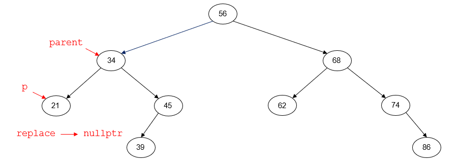
Node to delete has no left child

When a node we want to delete has no left child, we replace the deleted node with its right child. If the node to delete also has no right child, it will be replaced with nullptr.

For example, suppose that we want to delete the node with key 21. Prior to deleting the node, the tree will look like the following diagram. p points to the node to be deleted (21). parent points to the parent node of p (34). replace is set to p->right; since the node with key 21 has no right child, replace will be nullptr.

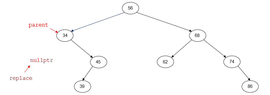
After deletion, the tree will look like this:

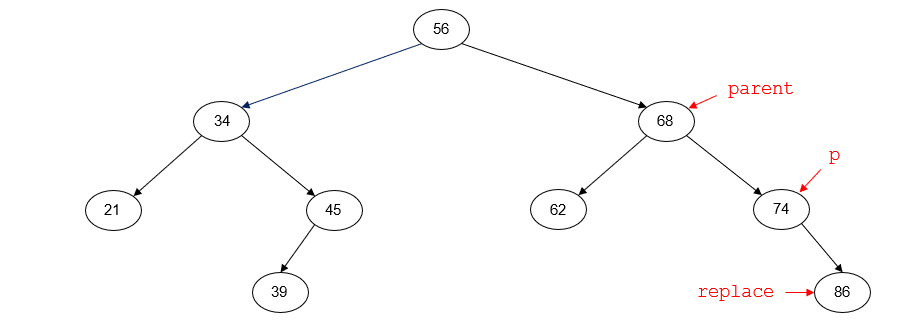
On the other hand, if the node we want to delete does have a right child, the deleted node is replaced with that right child.

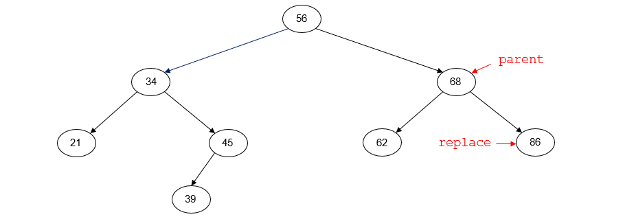
For example, suppose that we want to delete the node with key 74. Prior to deleting the node, the tree will look like the following diagram. p points to the node to be deleted (74). parent points to the parent node of p (68). replace points to the right child of p (86).

After deletion, the tree will look like this:
Node to delete has no right child

When a node we want to delete has no right child, we replace the deleted node with its left child.

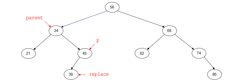
For example, suppose that we want to delete the node with key 45. Prior to deleting the node, the tree will look like the following diagram. p points to the node to be deleted (45). parent points to the parent node of p (34). replace points to the left child of p (39).

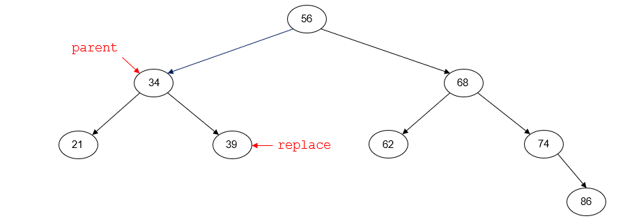
After deletion, the tree will look like this:
Node to delete has two children

When a node to delete has no right child, we replace the deleted node with its inorder predecessor. (Replacing the node with its inorder successor would also work, but we have to pick one or the other when we code the algorithm.) To find the inorder predecessor of a node with two children, we go to its left and then all the way to the right.

Sometimes after going left we may be unable to go right, because the left child of p has no right child. In that case, the left child of p is its inorder predecessor.

For example, suppose that we want to delete the node with key 68. Prior to deleting the node, the tree will look like the following diagram. p points to the node to be deleted (68). parent points to the parent node of p (56). replace points to the left child of p (62), which is its inorder predecessor. replace_parent points to the same node as p (68), which tells us that after going left we were unable to go to the right.

We know in this situation that the node pointed to by replace is the left child of p, so we don't need to worry about dealing with that. The node pointed to by p also has a right child. Since the node pointed to by replace currently has no right child of its own (remember, we were unable to go to the right), the right child of the node pointed to by p can become its new right child.

After deletion, the tree will look like this:

If the left child of p has a right child, we need to continue going to the right until we reach a node with no right child. That node will be the inorder predecessor of p.

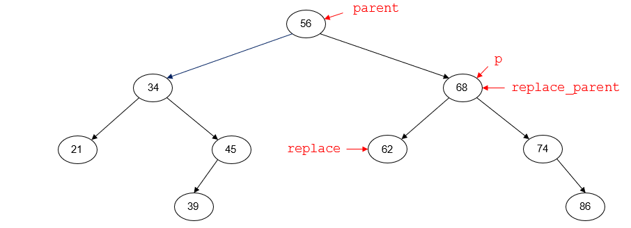
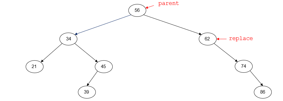
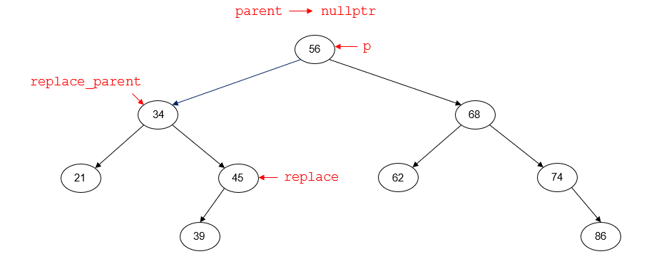
For example, suppose that we want to delete the node with key 56. Prior to deleting the node, the tree will look like the following diagram. p points to the node to be deleted (56). parent is nullptr; the node with key 56 is the root node of the tree and has no parent node. replace points to the inorder predecessor of p (45). replace_parent points to the parent node of replace (34).

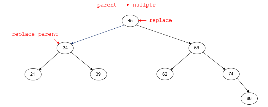
In this situation, we have a couple more links that need to be set. The node pointed to by replace has no right child, but it might have a left child. That left child will become the right child of replace_parent, taking the place of the node pointed to by replace.

The node pointed to by p definitely has both a left child and a right child - if it didn't, we wouldn't be in the code for this case! Those children need to become the children of the node pointed to by replace.

After deletion, the tree will look like this:

Binary Search Tree Find / Lookup

The find or lookup operation can be coded either iteratively or recursively. Pseudocode for an iterative version of this algorithm is shown below.

procedure find(key : a key for which to search)
    // root   : pointer to the root node of the tree (nullptr if tree is empty)
    // p      : pointer to a tree node
    
    // Start at the root of the tree.
    p ← root
    
    // Search the tree for a null link or a matching key.
    while p != nullptr and key != p->key
        if key < p->key
            p ← p->left
        else
            p ← p->right
        end if
    end while

    // p either points to the node with a matching key or is nullptr if 
    // the key is not in the tree.
    return p

end procedure

Alternatively, this algorithm can simply return true if the search key is found, and false if it is not found.

C++ Implementation of a Binary Search Tree

We can code a linked binary search tree as a struct and a class in C++.

Sample template struct to represent a tree node

template <class K, class V>
struct node
{
    K key;
    V value;
    node<K, V>* left;
    node<K, V>* right;
    
    node(const K& key = K(), const V& value = V(), node<K, V>* left = nullptr, node<K, V>* right = nullptr)
    {
        this->key = key;
        this->value = value;
        this->left = left;
        this->right = right;
    }
};

Class to represent a binary search tree

Data members

node<K, V>* root - Root pointer. Points to the root node of the tree or is nullptr if the tree is empty.
t_size - Tree size. The number of items currently stored in the binary search tree.

Member Functions

The insert(), remove(), and find() have already been described in detail. Any of the binary tree traversals (particularly inorder traversal) may be also be coded as member functions of the class. Other common member functions are described below.

Default constructor

Sets tree to initial empty state. The root node pointer should be set to nullptr. The tree size should be set to 0.
size()

Returns the tree size.
empty()

Returns true if the tree size is 0; otherwise, false.

clear()

Sets the tree back to the empty state.

procedure clear()    
    destroy(root)
    root ← nullptr;
    t_size ← 0
end procedure

destroy()

Recursively deletes the nodes of a bstree object. This is a modified version of a postorder traversal of the tree.

procedure destroy(p : pointer to a tree node)
    
    if p != nullptr

        // Recursively destroy the left and right subtrees of the node pointed to by p.
        destroy(p->left)     
        destroy(p->right)

        Delete the node pointed to by p
    end if
end procedure

Copy Constructor

procedure bstree(x : reference to a constant bstree)
    // Copy the other bstree object's size
    t_size ← x.t_size

    // Copy the nodes of the other bstree object
    root = clone(x.root)
end procedure

Copy Assignment Operator

procedure operator=(x : reference to a constant bstree)
    if this != &x
        // Make the left bstree object empty
        clear()
        
        // Copy the other bstree object's size
        t_size ← x.t_size

        // Copy the nodes of the other bstree object
        root = clone(x.root)
    end if
        
    return *this;
end procedure

Destructor

We can delete all of the dynamic storage for the tree by calling the clear() member function.

clone()

Recursively copies the nodes of a bstree object. This is a modified version of a preorder traversal of the tree.

procedure clone(p : pointer to a tree node)
    
    if p != nullptr

        // Make a copy of the node pointed to by p.
        Allocate a new tree node, new_node
        new_node->key ← p->key     
        new_node->value ← p->value
        
        // Recursively copy the left and right subtrees of the node pointed to by p.
        new_node->left ← clone(p->left)     
        new_node->right ← clone(p->right)
        
        return new_node 
    else
        return nullptr           
    end if
end procedure

Complexity

The time complexity for the insertion, deletion, and find / lookup operations is based on the height of the binary search tree. For a complete or almost complete binary tree, the time complexity of these operations will be O(log n) - we eliminate one of a node's two subtrees from consideration with each key comparison. In the case of a degenerate binary search tree, the time complexity of these operations will be no better than they would be for a linked list - i.e., O(n).

Space complexity for the iterative implementations of these operations will be O(1). For recursive implementations, the space complexity will be similar to the time complexity.

The time complexity for traversals of the tree will always be O(n), since we "visit" every node in the tree. This also includes the clone() and destroy() functions described above, which are called by the copy constructor, copy assignment operator, and destructor.

Space complexity for traversals of the tree is generally based on the height of the tree. For a complete or almost complete binary tree, the space complexity of a traversal will be O(log n), while a traversal of a a degenerate binary search tree will have a space complexity of O(n).